
Quick Start Guide to Neural Networks in R with Keras and Tensorflow
I’ve been working with neural networks lately and have struggled to find any quick start resources for getting up and running in R. To help others in a similar situation, I’m providing this quick start guide. It’s designed to help you get your first model up and going, enabling you to iterate quickly with your own data.
Introduction
Neural networks, a crucial part of machine learning, emulate the human brain’s network of neurons to process and learn from data. They are exceptionally adept at handling complex tasks such as pattern recognition, image and speech processing, natural language processing (NLP), time series prediction, and various classification challenges. This guide offers a hands-on example of how to use neural networks in R with {Keras} and {TensorFlow}, covering everything from data creation to model training and evaluation, specifically tailored for those looking to apply neural networks to tabular data.
Prerequisites
Since {Keras} is a Python-based package, you’ll need to ensure you have Python installed. You can download Python from the official Python website. After setting up Python, you’ll need to install Keras and {TensorFlow} in R. The following explanation, taken from the {Keras} documentation, details the installation process:
This function will install Tensorflow and all Keras dependencies. This is a thin wrapper around
tensorflow::install_tensorflow(), with the only difference being that this includes by default additional extra packages that keras expects, and the default version of tensorflow installed byinstall_keras()may at times be different from the default installed byinstall_tensorflow().
install.packages("keras")
install_keras()
Example for Tabular Data
Now, let’s start by creating some sample synthetic data for a neural network in R. We will use the keras package, a high-level neural networks API running on top of TensorFlow, which is a powerful open-source software library for machine learning.
Create Sample Data
I will create reproducible synthetic data to simulate a real-world dataset. This should allow you to have the same data on your compute as you follow along.
Notice how in this data I have centered and scaled the continuous covariates. This is a must for your neural network.
library(tidyverse)

set.seed(0)  # For reproducibility

n_samples <- 10000

# The bias term here is used to adjust the distribution of the binary outcome.
bias = -log(.001)

# Generate data
data <- tibble(
  factor_1 = rnorm(n_samples),  # Normally distributed data
  factor_2 = rnorm(n_samples, mean = 5, sd = 2) + 0.5 * factor_1,  # Correlated with factor_1
  factor_3 = runif(n_samples, min = -1, max = 1),  # Uniformly distributed data
  factor_4 = rbinom(n_samples, size = 10, prob = 0.5),  # Binomially distributed data
  factor_5 = factor_3 * factor_4,  # Interaction term
  factor_6 = sample(0:1, n_samples, replace = TRUE)  # Binary data
) |>
  # The outcome is a binary variable created using a logistic function (plogis)
  # of the factors, which simulates a complex relationship.
  mutate(outcome = rbinom(n(), 1,
                          prob = plogis(factor_1 - 2 * factor_2 + factor_3 * factor_4 -
                                          factor_5 + factor_6 + bias)
                          )
         ) |>
  mutate(across(.cols = c(factor_4, factor_6, outcome), .fns = as.factor)) |>
  mutate(across(.cols = is.numeric, .fns = ~(.-mean(.)/sd(.)))) |>
  mutate(across(.cols = everything(), .fns = ~as.numeric(as.character(.))))
Outcome Percentage
We can see a fairly reasonable split of the outcome in this data.
| outcome | Percent |
|---|---|
| 0 | 72.13% |
| 1 | 27.87% |
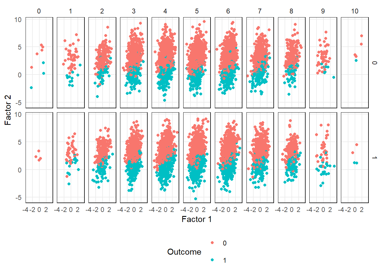
Visualize Data
From the plot below, you can see the the relationship a select number of factors has with the outcome.
Neural Network
Split into Test and Train
library(keras)

set.seed(0)

split_index <- sample(1:nrow(data), size = 0.8 * nrow(data))
train_data <- data[split_index, ]
test_data <- data[-split_index, ]
Define the Model Architecture
model <- keras_model_sequential() |>
  layer_dense(units = 100, activation = 'relu', input_shape = ncol(train_data) - 1) |>
  layer_dense(units = 100, activation = 'relu') |>
  layer_dense(units = 1, activation = 'sigmoid')
Model Architecture Details
Hidden Layers: The model includes two hidden layers, each with 100 neurons and using the ‘relu’ (Rectified Linear Unit) activation function. Alternatives to ‘relu’ include ‘tanh’ and others, each having its own merits depending on the specific use case.
Output Layer: The final dense layer makes the predictions. I use a ‘sigmoid’ activation function here, which is ideal for binary classification tasks as it returns values between 0 and 1, indicating the probability of the target class.
Input Shape: The
input_shapein the first layer is set to match the number of predictor columns in the data. This ensures that the model correctly processes the input features.Sequential Model: I’ve chosen a sequential model for its simplicity and effectiveness in stacking layers linearly. However, other options like functional API models exist, which allow for more complex architectures.
Selecting the Best Options
Choosing the optimal structure and functions for your neural network involves balancing several factors:
Data Characteristics: Understanding the shape, size, and type of your data is fundamental. Different data types might require different network architectures.
Modeling Objective: What you are trying to predict or classify directly influences your choice of architecture and activation functions.
Complexity of Relationships: The complexity in your data’s relationships can dictate the depth and complexity of the neural network required.
Experience and Experimentation: Selecting the best model is a cross between your own experience and experimentation. Running several models with different configurations and analyzing their performance is the best approach though the cost is the time it takes to run the models.
Advanced Layer Types: For certain types of data, especially sequential data like time series or text, using advanced layer types such as Long Short-Term Memory (LSTM) (for time series) or Convolutional Neural Networks (CNNs) might be beneficial (text, imagery).
Compile the Model
The next block of code “compiles” the model and configures it for training. It sets up up the optimizer, loss function, and metrics:
model |> compile(
  optimizer = 'adam',
  loss = 'binary_crossentropy',
  metrics = c('accuracy',
              metric_precision(),
              metric_recall())
)
Understanding the Compile Configuration
- Optimizer (
optimizer = 'adam'):- The optimizer is responsible for updating the weights of the neurons during training.
- The ‘adam’ optimizer is a popular choice due to its efficiency with large datasets and high-dimensional spaces.
- Alternatives like ‘sgd’ (Stochastic Gradient Descent) and ‘rmsprop’ are also available, each suited to different types of problems.
- Loss Function (
loss = 'binary_crossentropy'):- This function quantifies the difference between the expected outcome and the predictions made by the model.
- Binary Crossentropy (log loss) is works well for for binary classification.
- Other options include ‘mean_squared_error’ for regression tasks and ‘categorical_crossentropy’ for multi-class classification.
- Metrics:
- Metrics are used to evaluate the performance of the model. They are not used in the training process but provide insight into how well the model is performing.
metric_accuracy()assesses the overall correctness of the predictions.metric_precision()measures the proportion of positive identifications that were actually correct.metric_recall()calculates the proportion of actual positives that were correctly identified.- Other metrics include but are not limited to
metric_mse()(mean squared error),metric_mae()(mean absolute error), andmetric_auc().
Selecting the right combination of these parameters should reflect the specific characteristics of your data and the problem you are solving.
Fitting the Model
The following code block is for fitting (training) the neural network model. It specifies the training data, number of training cycles (epochs), and other important parameters:
history <- model |> fit(
x = as.matrix(train_data[,-7]),
y = as.matrix(train_data[,7]),
epochs = 20,
batch_size = 100,
validation_split = 0.3,
verbose = FALSE
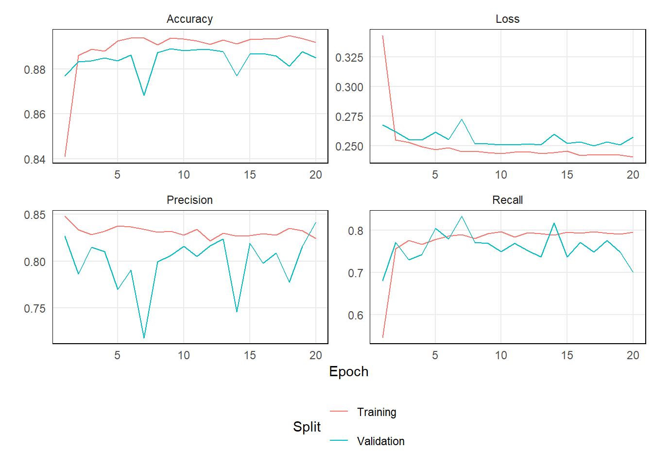
)Below is a look at the model’s metrics by epoch.
Understanding the Model Training Configuration
- x/y:
- These represent the training and test sets, respectively.
- The
x(features) must be in a format acceptable by the model, typically a matrix or array in numerical format. The number of columns inxshould match the number of input features the model expects. - The
y(target) also needs to be in a numerical format, either as a vector for regression or binary classification, or as a one-hot encoded matrix for multi-class classification.
- Epochs (
epochs = 20):- An epoch represents one complete pass through the entire training dataset. Here, the model will go through the dataset 20 times.
- The more epochs, the longer the model has to learn the data. However, there’s a risk of overfitting to the training set. This can be mitigated with techniques such as regularization, dropout between layers, and model callbacks, which are not included in this example.
- Batch Size (
batch_size = 100):- This defines the number of samples that will be propagated through the network in one pass. A smaller batch size means less memory usage but potentially less accurate estimation of gradients. I recommended you use as large of a batch size as your computer can handle and you have patience for.
- Validation Split (
validation_split = 0.3):- This parameter reserves a portion of the training data (30% in this case) for validation. The model’s performance on this validation set provides a good indication of its generalization to unseen data.
- Verbose (
verbose = FALSE):- This controls the level of verbosity of the training process output. It is set to
FALSEhere to suppress the progress messages for each epoch. This is done to avoid cluttering the description, but I recommended you set it toTRUEto follow its progress.
- This controls the level of verbosity of the training process output. It is set to
The fit function tunes the model to your data by adjusting the weights. The history object captures details about the training process, which can be used for further analysis and understanding of the model’s performance over time.
Make Predictions
We can make predictions using the standard predict() method.
test_data_w_preds <-
test_data |> mutate(predictions = predict(model, as.matrix(test_data[,-7]), verbose = 0)[,1]) |>
  mutate(binary_prediction = as.factor(ifelse(predictions > .5,1,0)))
Evaluating the Model
We can find the accuracy, prediction, and recall using {keras} or…
out <- model |> evaluate(as.matrix(test_data[,-7]), test_data[,7]$outcome, verbose = FALSE)
out
## loss accuracy precision recall
## 0.2474161 0.8903770 0.8597701 0.7003745…using {yardstick}.
library(yardstick)
classification_metrics <- metric_set(accuracy, precision, recall)

test_data_w_preds |>
  mutate(outcome = as.factor(outcome)) |>
  classification_metrics(truth = outcome, estimate = binary_prediction) |>
  gt::gt() |>
gt::fmt_percent(columns = .estimate)| .metric | .estimator | .estimate |
|---|---|---|
| accuracy | binary | 88.95% |
| precision | binary | 89.78% |
| recall | binary | 95.84% |
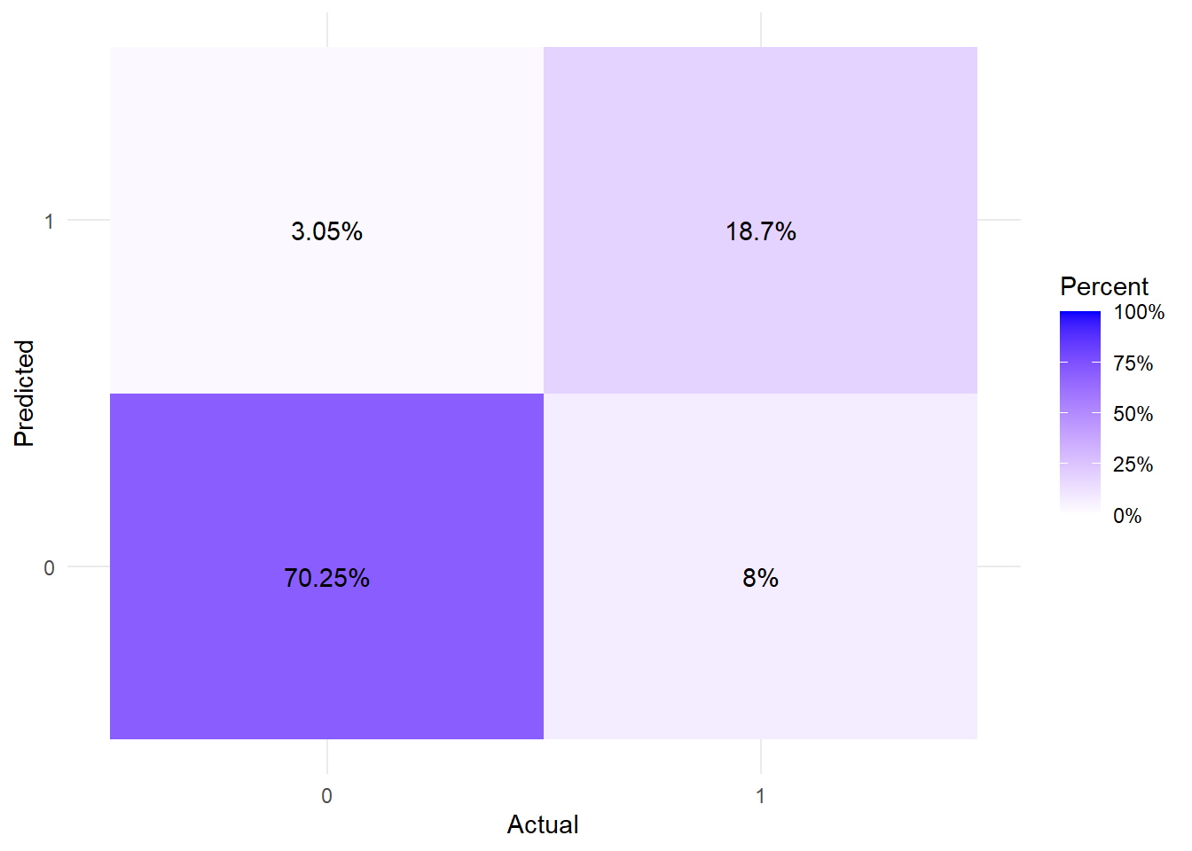
And a vew at the confusion matrix for good measure.
That’s a Wrap
I’ve tried to provide step-by-step introductions to implement a neural network for in R using the {Keras} package. We walked through generating reproducible sample data, defining a simple neural network architecture, training the model, making predictions on new data, and evaluating model performance. This guide should equip beginners with the initial skills needed to start building and applying neural networks to their own tabular data.
While neural networks can appear complex, breaking the process down into digestible steps makes them more accessible. With the right data preprocessing, model configuration, training parameters and performance metrics, neural networks can be powerful tools for tackling complex data patterns. The R ecosystem, with packages like {Keras} and {Tensorflow}, provides a convenient platform for leveraging the strengths of neural networks. By following this guide and adjusting the components to their specific use case, you should now (hopefully) be able to start neural network modeling in R.