Introduction
Over Christmas 2017, my wife, Jill, resolved that our family (to include babysitters) would read our children over 1000 new books in 2018. More specifically, 29 December 2017 - 28 December 2018.
A goal like this takes dedication, love, and of course, a Data Science-y approach.
Special thanks to Ally, Zia, and Bookbuddy for help in accomplishing this goal!
Also, special thanks to drob and juliasilge who privde the tidytext package and the entire R open-source community I rely on to do this analysis.
Since I use this page as a way to log my ideas and teach others (and future me) how I did this, I’ll include the code.
Exploratory Data Analysis
Libraries
The libraries I will use for this analysis are the following:
library(tidyverse)
library(lubridate)
library(janitor)
library(stringr)
library(tidytext)
library(forcats)
library(zoo)
library(kableExtra)
library(DT)
Read in Data
Lets read in the data and get a feel for what information we have. Since my wife, our babysitter, and I have scanned the books in bookbuddy, I need to upload all the data and join it together. We have the data in many different spreadsheets to I’ll have to read them all in separately. I had to change some of the columns to character to make joining these dataframes go more smooth later on.
book = read_csv("data/children_book/BookBuddy.csv") %>% mutate(ISBN = as.numeric(ISBN))
book1 = read_csv("data/children_book/BookBuddy (1).csv") %>% mutate(ISBN = as.numeric(ISBN)) %>% mutate(OCLC = as.character(OCLC)) %>% mutate(`Date Published` = mdy(`Date Published`)) %>% mutate(`Date Added` = as.character(`Date Added`))
book2 = read_csv("data/children_book/BookBuddy (2).csv") %>% mutate(ISBN = as.numeric(ISBN)) %>% mutate(OCLC = as.character(OCLC)) %>% mutate(`Date Published` = mdy(`Date Published`)) %>% mutate(`Date Added` = as.character(`Date Added`))
book3 = read_csv("data/children_book/BookBuddy (3).csv") %>% mutate(ISBN = as.numeric(ISBN)) %>% mutate(OCLC = as.character(OCLC)) %>% mutate(`Date Published` = mdy(`Date Published`)) %>% mutate(`Date Added` = as.character(`Date Added`))
book4 = read_csv("data/children_book/BookBuddy (4).csv") %>% mutate(ISBN = as.numeric(ISBN)) %>% mutate(OCLC = as.character(OCLC)) %>% mutate(`Date Published` = mdy(`Date Published`)) %>% mutate(`Date Added` = as.character(`Date Added`))
book5 = read_csv("data/children_book/BookBuddy (5).csv") %>% mutate(ISBN = as.numeric(ISBN)) %>% mutate(OCLC = as.character(OCLC)) %>% mutate(`Date Published` = mdy(`Date Published`)) %>% mutate(`Date Added` = as.character(`Date Added`))
book6 = read_csv("data/children_book/BookBuddy (6).csv") %>% mutate(ISBN = as.numeric(ISBN)) %>% mutate(OCLC = as.character(OCLC)) %>% mutate(`Date Published` = mdy(`Date Published`)) %>% mutate(`Date Added` = as.character(`Date Added`))
book7 = read_csv("data/children_book/BookBuddy (7).csv")  %>% mutate(ISBN = as.numeric(ISBN)) %>% mutate(OCLC = as.character(OCLC)) %>% mutate(`Date Published` = mdy(`Date Published`)) %>% mutate(`Date Added` = as.character(`Date Added`))
book8 = read_csv("data/children_book/BookBuddy (8).csv")  %>% mutate(ISBN = as.numeric(ISBN)) %>% mutate(OCLC = as.character(OCLC)) %>% mutate(`Date Published` = mdy(`Date Published`)) %>% mutate(`Date Added` = as.character(`Date Added`))
book9 = read_csv("data/children_book/BookBuddy (9).csv")  %>% mutate(ISBN = as.numeric(ISBN)) %>% mutate(OCLC = as.character(OCLC)) %>% mutate(`Date Published` = mdy(`Date Published`)) %>% mutate(`Date Added` = as.character(`Date Added`))
book10 = read_csv("data/children_book/BookBuddy (10).csv")  %>% mutate(ISBN = as.numeric(ISBN)) %>% mutate(OCLC = as.character(OCLC)) %>% mutate(`Date Published` = mdy(`Date Published`)) %>% mutate(`Date Added` = as.character(`Date Added`))
book11 = read_csv("data/children_book/BookBuddy (11).csv")  %>% mutate(ISBN = as.numeric(ISBN)) %>% mutate(OCLC = as.character(OCLC)) %>% mutate(`Date Published` = mdy(`Date Published`)) %>% mutate(`Date Added` = as.character(`Date Added`))
book12 = read_csv("data/children_book/BookBuddy (12).csv") %>% mutate(ISBN = as.numeric(ISBN)) %>% mutate(OCLC = as.character(OCLC)) %>% mutate(`Date Published` = mdy(`Date Published`)) %>%  mutate(`Date Added` = as.character(`Date Added`))
book13 = read_csv("data/children_book/BookBuddy (13).csv") %>% mutate(ISBN = as.numeric(ISBN)) %>% mutate(OCLC = as.character(OCLC)) %>% mutate(`Date Published` = mdy(`Date Published`)) %>% mutate(`Date Added` = as.character(`Date Added`))
book14 = read_csv("data/children_book/BookBuddy (14).csv") %>% mutate(ISBN = as.numeric(ISBN)) %>% mutate(OCLC = as.character(OCLC)) %>% mutate(`Date Published` = mdy(`Date Published`)) %>% mutate(`Date Added` = as.character(`Date Added`))
book15 = read_csv("data/children_book/BookBuddy (15).csv") %>% mutate(ISBN = as.numeric(ISBN)) %>% mutate(OCLC = as.character(OCLC)) %>% mutate(`Date Published` = mdy(`Date Published`)) %>% mutate(`Date Added` = as.character(`Date Added`))
Join and Clean Data
Now that we’ve read it in, I need to do a few things to support future analysis.
Many of the column names have spaces which does not support data munging. I’ll use the
clean_namescommand from thejanitorpackage to clean this up.I have a lot of duplicate books. I’ll keep only the rows that have distinct Title and Author. I used the
distinctcommand because some of us scanned the same books. We do not want to account for them twice.I need to convert the
DatePublishedandDateAddedto characters (don’t worry, I’ll bring it back later.)It seemed like every Berenstain Bear book had a little bit different Author. Lets clean that up a little too.
There were some
DateAddeddates that do not exist. For a while, when one of our babysitters was saving the data, this information was not being saved. We assigned the book the most recent data from when we caught the error (as seen in the last line below). This is not a reasonable assumption, but its the best we can do.Lastly, I’ll only use the following columns:
Title,Author,Publisher,YearPublished,Genre,Summary,DateAdded,DatePublished, andGoogleVolumeId. The rest of the columns contain blank information.
booksread =
  book %>% bind_rows(book1) %>% bind_rows(book2) %>% bind_rows(book3)  %>%
  bind_rows(book4) %>% bind_rows(book5) %>% bind_rows(book6) %>%
  bind_rows(book7) %>% bind_rows(book8) %>% bind_rows(book9) %>%
  bind_rows(book10) %>%  bind_rows(book11) %>% bind_rows(book12) %>%
  bind_rows(book13) %>% bind_rows(book14) %>% bind_rows(book15) %>%
  clean_names(case = "upper_camel") %>%
  distinct(Title, Author, .keep_all = TRUE) %>%
  mutate(DatePublished = ymd(str_sub(DatePublished,1,10)))%>%
  mutate(DateAdded = ymd(str_sub(DateAdded,1,10))) %>%
  select(Title, Author, Publisher, YearPublished, Genre, Summary, NumberOfPages, DateAdded, DatePublished,GoogleVolumeId) %>%
  mutate(Author = ifelse(grepl("Bere", Author)==TRUE, "Berenstein", Author)) %>%
  mutate(DateAdded = na.locf(.$DateAdded, fromlast = TRUE))
Here is the data for you to explore:
booksread %>%
  select(-Summary) %>%
  datatable()
Analysis
To answer the primary question: How many books did we read?
nrow(booksread)## [1] 1070What is the span of the dates of our our books?
booksread$DateAdded %>% min## [1] "2017-12-29"booksread$DateAdded %>% max## [1] "2018-12-18"Top Authors
What other interesting things can we find? Who were our top authors?
booksread %>%
  group_by(Author) %>%
  summarise(n = n()) %>%
  arrange(desc(n)) %>%
  filter(n>5) %>%
kable()| Author | n |
|---|---|
| Berenstein | 72 |
| Mercer Mayer | 17 |
| Dr. Seuss | 15 |
| James Dean | 14 |
| Victoria Kann | 14 |
| Cynthia Rylant | 11 |
| Jane O’Connor | 9 |
| Gail Gibbons | 6 |
| Kate Banks | 6 |
| Rosemary Wells | 6 |
booksread %>%
  group_by(Author) %>%
  summarise(n = n()) %>%
  filter(n>5) %>%
  ggplot(aes(x=fct_reorder(Author, desc(n)), y = n)) +
  geom_bar(stat = "identity") +
  labs(title = "Most Read Authors", x = "Authors", y = "Number of Books") +
  theme(axis.text.x = element_text(angle = 45, hjust = 1))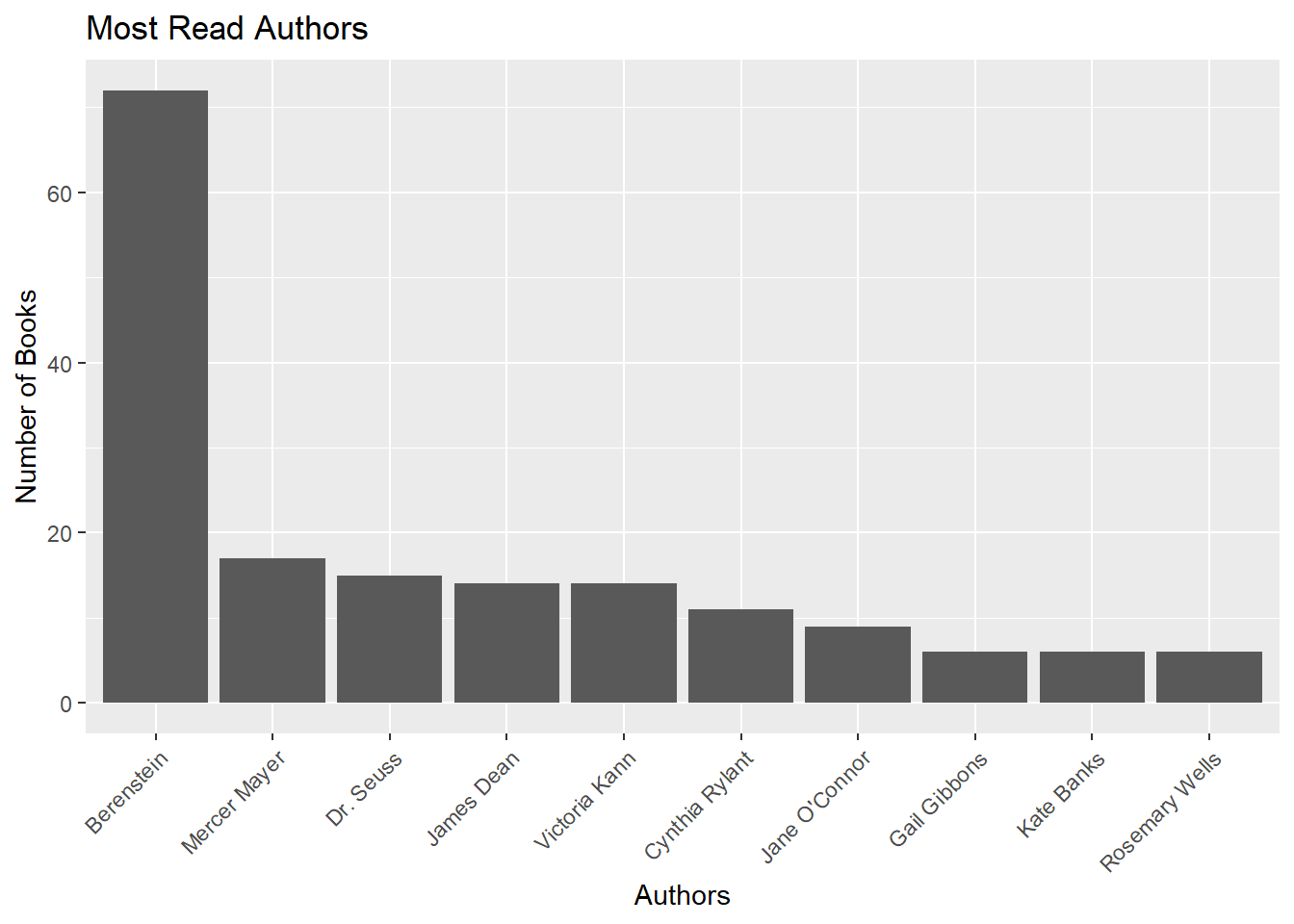
I’m a big fan of the Berenstain Bears, Dr. Seuss, and Pete The Cat (James Dean), but not so much Fancy Nancy (Thanks Jane O’Connor)….
Timeline
booksread %>%
  group_by(DateAdded) %>%
  summarise(n = n()) %>%
  ungroup() %>%
  mutate(BooksByDate = cumsum(n)) %>%
  ggplot(aes(x=DateAdded, y = BooksByDate)) +
  geom_line() +
  geom_point() +
  labs(title = "Books Read in 2018", x = "Date", y = "Total Books Read")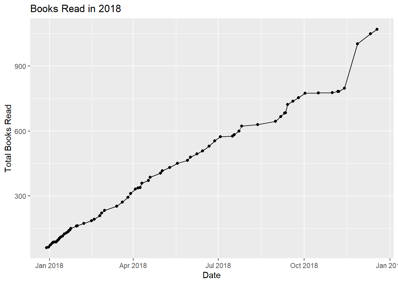
There are a few things to note from the data above.
We were more vigilant at scanning books as we read them at the beginning – vs scanning them all at once at the end.
We had a couple droughts of book reading – in particular August was a slow period.
The big jump in December was a data collection error mentioned above. These were likely spread across the previous 3 months.
booksread %>%
  mutate(month = month(DateAdded)) %>%
  group_by(month) %>%
  summarise(BooksInMonth = n()) %>%
kable()| month | BooksInMonth |
|---|---|
| 1 | 98 |
| 2 | 59 |
| 3 | 90 |
| 4 | 95 |
| 5 | 58 |
| 6 | 90 |
| 7 | 69 |
| 8 | 22 |
| 9 | 109 |
| 10 | 23 |
| 11 | 225 |
| 12 | 132 |
A Book by… God?
And just as a side note, I happen to see we had a book authored by ‘God’. Lets investigate.
booksread %>%
  filter(Author=="God") %>%
  select(Title, Author) %>%
kable()| Title | Author |
|---|---|
| The Lord’s prayer | God |
Okay then.
Publication Date
When were our books published?
ggplot(data = booksread, aes(YearPublished)) +
  geom_bar() +
  labs(title = "Books By Year", y = "Total Books", x = "Year Published")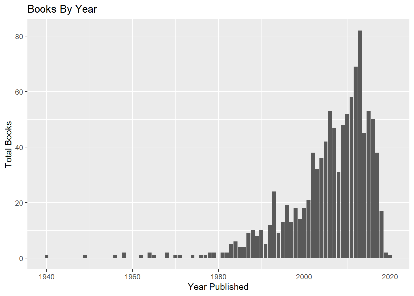
It appears we’ve read some classics… as well as some of the more ‘pop culture’ children’s books.
Length of Books
I can hear you now…“So you’ve read over 1000 books this year. Its nice that they are all picture books…”"
ggplot(data = booksread, aes(NumberOfPages)) +
  geom_histogram() +
  ggtitle("Books By Number of Pages") + ylab("Total Books")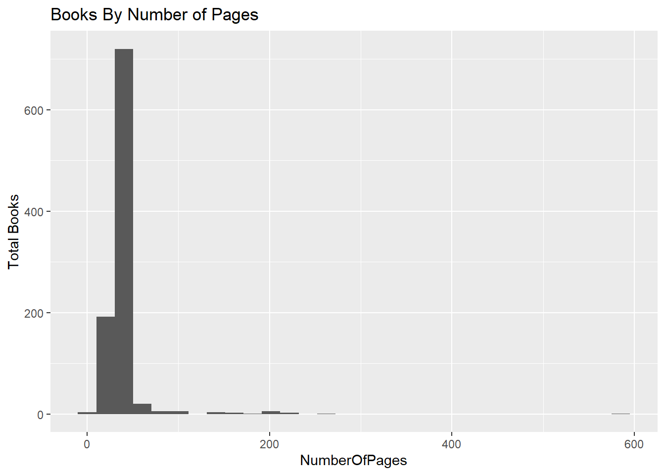
What?! We’ve read books over 100 pages to our kids…
booksread %>%
  filter(NumberOfPages>100) %>%
  arrange(desc(NumberOfPages)) %>%
  select(Title, Author, NumberOfPages) %>%
kable()| Title | Author | NumberOfPages |
|---|---|---|
| Disney’s Once Upon a Princess | Various, | 592 |
| Brick City | Warren Elsmore | 256 |
| The Curious Kid’s Science Book | Asia Citro | 224 |
| Good Night Stories for Rebel Girls | Elena Favilli, Francesca Cavallo | 212 |
| LEGO Adventure Book, Vol. 1 | Megan H. Rothrock | 200 |
| The LEGO Ideas Book | Daniel Lipkowitz | 198 |
| Lots of Look & Finds Disney Princess | Author | 193 |
| Little Critter’s Read-it-yourself Storybook | Mercer Mayer | 192 |
| Pinkalicious: The Pinkamazing Storybook Collection | Victoria Kann | 192 |
| Space Encyclopedia | Christine Pulliam, Patricia Daniels | 191 |
| My Friend the Moon | André Dahan | 160 |
| Big Book of the Berenstain Bears | Berenstein | 160 |
| Yoga games for children | Danielle Bersma | 146 |
| Yoga Games for Children | Danielle Bersma, Marjoke Visscher | 146 |
| The LEGO Build-It Book, Vol. 1 | Nathanael Kuipers, Mattia Zamboni | 132 |
Book Genres
What types of books do we read our kids?
It appears a pretty interesting array of genres. And some uniquely named ones if you search around.
booksread %>%
  filter(!is.na(Genre)) %>%
  group_by(Genre) %>%
  summarise(n = n()) %>%
  arrange(desc(n)) %>%
  datatable()
Text Analysis
So, that was some interesting descriptive analysis. Lets look at the undertones our children are absorbing from what we are reading.
I’d really like to know what type of words / sentiment we are reading our children – but until I can figure out a way to get the words from all the books, I’ll have to rely on the Summary provided by BookBuddy.
Here’s an example of what we’ll be looking at:
booksread %>%
  filter(Title=="Mama Cat Has Three Kittens") %>%
  select(Summary)
## # A tibble: 1 x 1
## Summary
## <chr>
## 1 Some kittens march to the beat of a different drummer.Mama Cat has three kittens, Fluffy, Skinny, and Boris. Where Mama Cat leads, Fluffy and Skinn~Preparation
So, lets prepare the data. I’d like to bring along some information while I tokenize the summaries (Titles, Authors, and Genres).
text_df = data_frame(line = 1:length(booksread$Summary), text = as.character(booksread$Summary), book = booksread$Title, Genre = booksread$Genre, Author = booksread$Author)

cleanedbooks = text_df %>%
  unnest_tokens(word, text) %>%
  anti_join(stop_words, by = "word")

cleanedbooks %>% datatable()
In this process, I’d like to note several things:
I removed “stop words” – words such as ‘a’, ‘an’, ‘the’ and many other words that do not contain sentiment.
In order to classify the text, I’ll rely on the NRC data base. Using this database, I’ll assign emotion to many words to determine the sentiment of what we’ve been reading our children.
I’ll also like to translate NRCs emotions into
Positive,Negative, andNeutralclassifications.I also recognize that some of the words are double counted using this technique. For example the word “joyful” is classified 3 times (as joy, positive, and trust). I will make the assumption that words like this are stronger and therefore these multi-counts will account for the added emphasis.
nrcbooks = cleanedbooks %>%
  inner_join(get_sentiments("nrc"), by = "word") %>%
  mutate(sent = ifelse(sentiment=="joy"|sentiment=="positive"|sentiment=="suprise"|sentiment=="trust","Positive Words",
                       ifelse(sentiment=="disgust"|sentiment=="fear"|sentiment=="negative"|sentiment=="sadness","Negative Words","Neutral Words"))) %>%
  mutate(sent = as.factor(sent))
In the table below, you can see an example of the words in each book and the assigned sentiment to each word.
nrcbooks %>%
  head(15) %>%
kable()| line | book | Genre | Author | word | sentiment | sent |
|---|---|---|---|---|---|---|
| 1 | And Then Comes Summer | Juvenile Fiction | Tom Brenner | joyful | joy | Positive Words |
| 1 | And Then Comes Summer | Juvenile Fiction | Tom Brenner | joyful | positive | Positive Words |
| 1 | And Then Comes Summer | Juvenile Fiction | Tom Brenner | joyful | trust | Positive Words |
| 1 | And Then Comes Summer | Juvenile Fiction | Tom Brenner | sun | anticipation | Neutral Words |
| 1 | And Then Comes Summer | Juvenile Fiction | Tom Brenner | sun | joy | Positive Words |
| 1 | And Then Comes Summer | Juvenile Fiction | Tom Brenner | sun | positive | Positive Words |
| 1 | And Then Comes Summer | Juvenile Fiction | Tom Brenner | sun | surprise | Neutral Words |
| 1 | And Then Comes Summer | Juvenile Fiction | Tom Brenner | sun | trust | Positive Words |
| 1 | And Then Comes Summer | Juvenile Fiction | Tom Brenner | tribute | positive | Positive Words |
| 1 | And Then Comes Summer | Juvenile Fiction | Tom Brenner | anticipation | anticipation | Neutral Words |
| 1 | And Then Comes Summer | Juvenile Fiction | Tom Brenner | yawn | negative | Negative Words |
| 1 | And Then Comes Summer | Juvenile Fiction | Tom Brenner | cheerful | joy | Positive Words |
| 1 | And Then Comes Summer | Juvenile Fiction | Tom Brenner | cheerful | positive | Positive Words |
| 1 | And Then Comes Summer | Juvenile Fiction | Tom Brenner | cheerful | surprise | Neutral Words |
| 1 | And Then Comes Summer | Juvenile Fiction | Tom Brenner | jump | joy | Positive Words |
Total Sentiment
Lets look at the sentiment my children are receiving in their books (as told by the summaries)
ggplot(data = nrcbooks, aes(sent, color = sentiment, fill = sentiment)) +
  geom_bar() +
  ggtitle("Type of Words in my Children's Books") + xlab("Sentiment") + ylab("Total Count")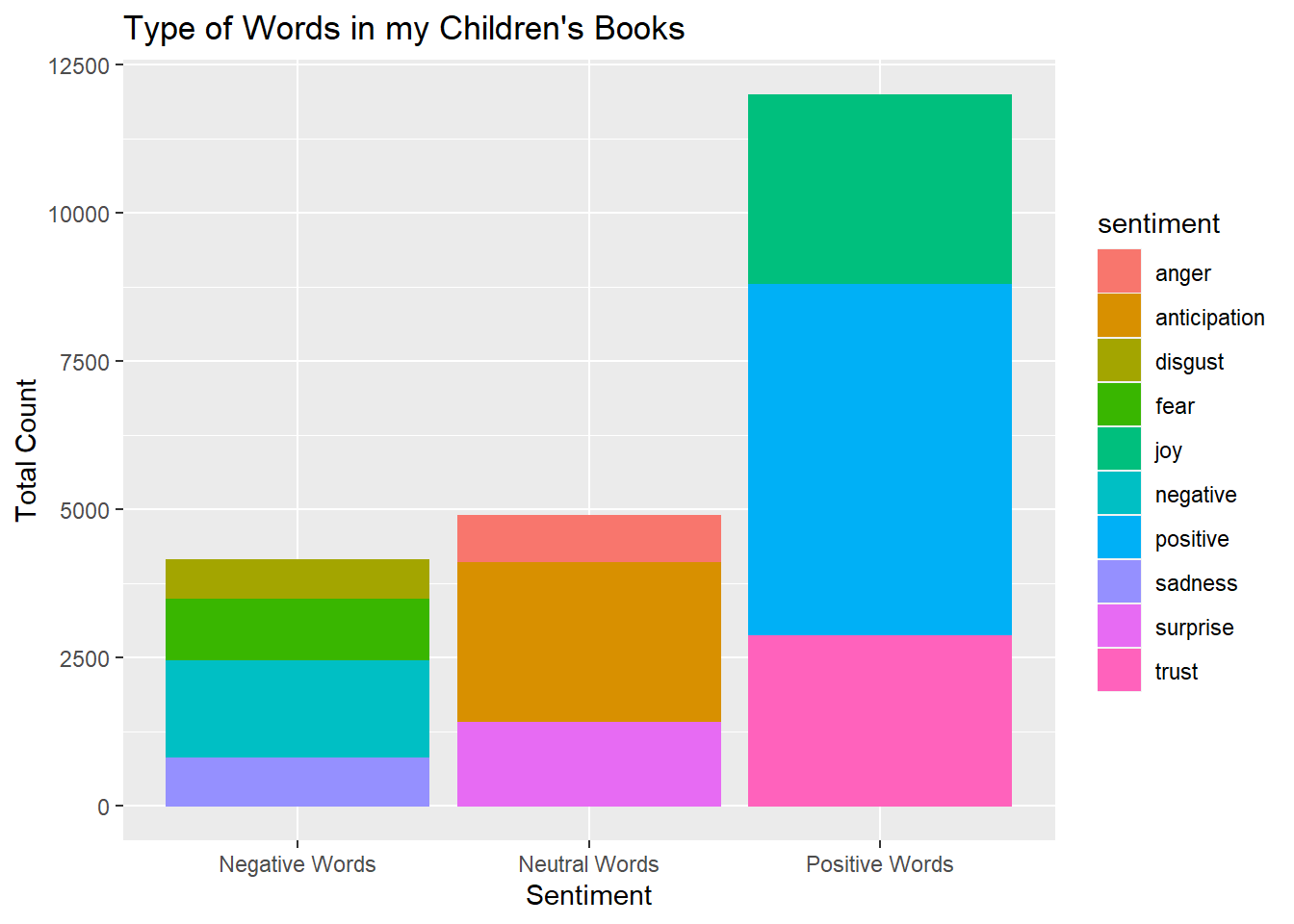
It looks like, as far as the summaries indicate, that our kids are hearing positive words.
Sentiment By Authors
Lets see which authors provide more sentiment.
nrcbooks %>%
  mutate(sent = case_when(sent == "Positive Words" ~ 1,
                          sent == "Neutral Words" ~ 0,
                          sent == "Negative Words" ~ -1)) %>%
  group_by(Author) %>%
  summarise(NetSentiment = sum(sent)/sum(abs(sent)), TotalSent = n()) %>%
  datatable()
Lets take a look visually.
nrcbooks %>%
  group_by(Author) %>%
  add_tally() %>%
  filter(n>160) %>%
ggplot(aes(sent, color = sentiment, fill = sentiment)) +
  geom_bar() +
  facet_wrap("Author", scales = "free_y") +
  ggtitle("Type of Words my Children Listen to in Books") + xlab(" ") + ylab("Total Count")  +
  theme(axis.text.x = element_text(angle = 45, hjust = 1))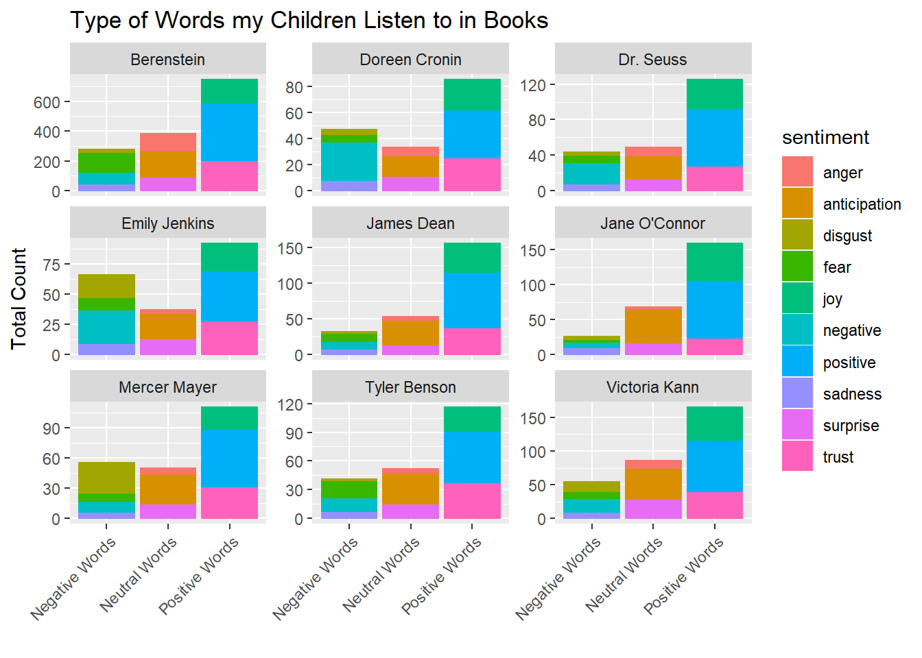
Sentiment by Genre
Lets see if there’s a genre that has any sentiment sway. Of note, I find it funny that there is a ‘Bears’ genre.
nrcbooks %>%
  group_by(Genre) %>%
  add_tally() %>%
  filter(!is.na(Genre)) %>%
  filter(n>100) %>%
ggplot(aes(sent, fill = sent)) +
  geom_bar() +
  facet_wrap("Genre", scales = "free_y") +
  ggtitle("Sentiment by Genre") + xlab("Sentiment")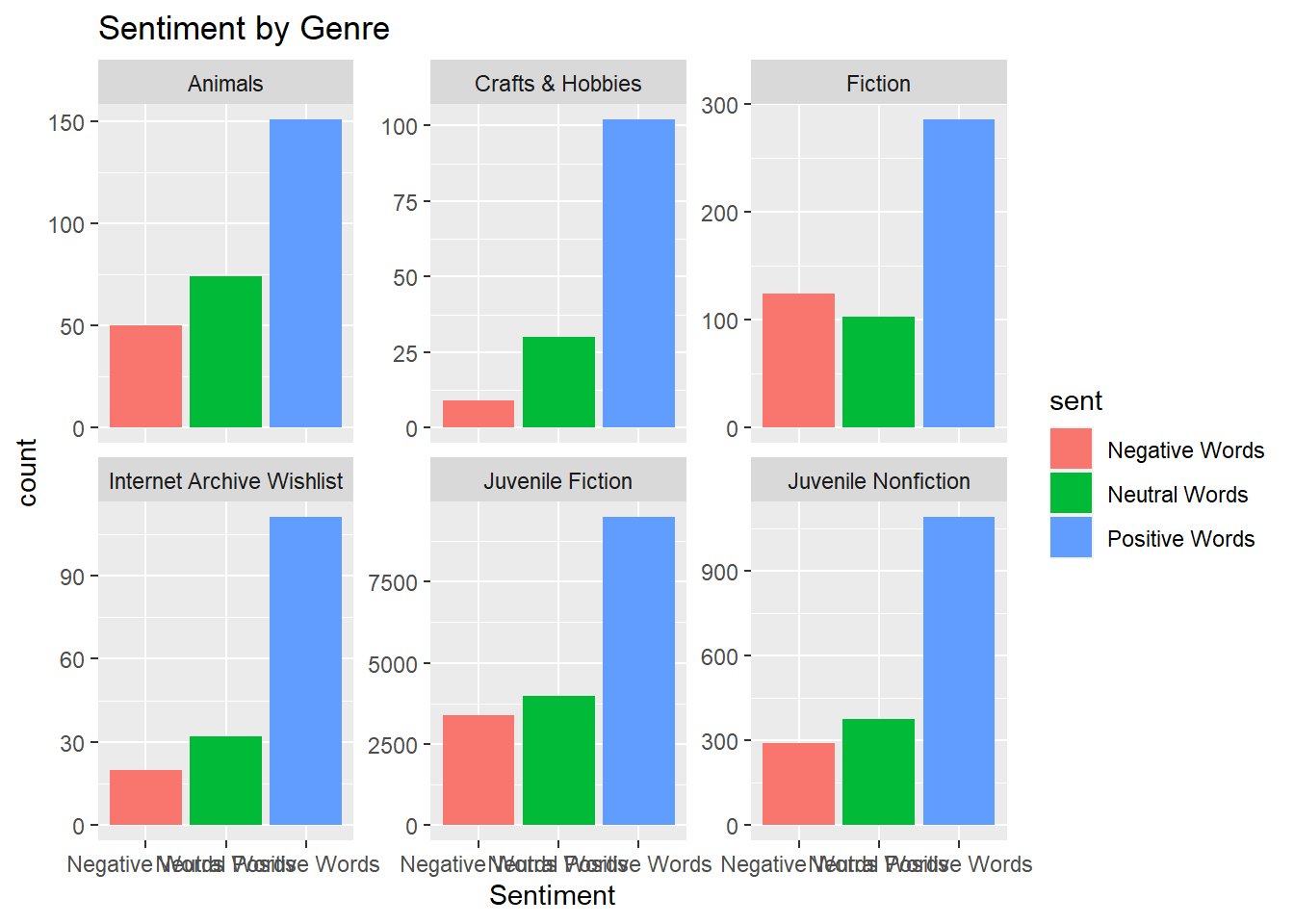
Happiest and Saddest Book
My wife remembers being in tears in a couple of books she read our kids. I’ll filter for ‘sad’ words to make this determination.
nrcbooks %>%
  filter(sentiment == "sadness") %>%
  group_by(book, Author) %>%
  summarise(n = n()) %>%
  filter(n>5) %>%
  arrange(desc(n)) %>%
  kable()
## `summarise()` has grouped output by 'book'. You can override using the `.groups` argument.| book | Author | n |
|---|---|---|
| Snap! | Hazel Hutchins | 8 |
| Have You Seen My New Blue Socks? | Eve Bunting | 7 |
| The Day the Crayons Came Home | Drew Daywalt | 7 |
| The Legend of the Poinsettia | Tomie De Paola | 7 |
| The Night Pirates | Peter Harris | 7 |
| A Fine Dessert | Emily Jenkins | 6 |
| Black Cat & White Cat | Claire Garralon | 6 |
| Boo Hoo Bird | Jeremy Tankard | 6 |
| Butterfly Tree | Sandra Markle | 6 |
| Hedgehog, Pig, and the Sweet Little Friend | Lena Anderson | 6 |
| Snowflakes Fall | Patricia MacLachlan | 6 |
Thought it doesn’t show up here, “Big Cat, Little Cat” is a very sad book (according to my wife).
Lets see if we can find it.
nrcbooks %>%
  filter(grepl("Cat",book)==TRUE) %>%
  filter(sentiment == "sadness") %>%
  group_by(book, Author) %>%
  summarise(n = n()) %>%
  filter(n>1) %>%
  arrange(desc(n)) %>%
  kable()
## `summarise()` has grouped output by 'book'. You can override using the `.groups` argument.| book | Author | n |
|---|---|---|
| Black Cat & White Cat | Claire Garralon | 6 |
| Hero Cat | Eileen Spinelli | 5 |
| Drat that Fat Cat! | Pat Thomson | 4 |
| KokoCat, Inside and Out | Lynda Graham-Barber | 4 |
| Pete the Cat and His Magic Sunglasses | James Dean, Kimberly Dean | 4 |
| Pete the Cat and the Bad Banana | James Dean | 4 |
| Big Cat, Little Cat | Elisha Cooper | 2 |
| Fat Cat | Margaret Read MacDonald | 2 |
| Gracie the Lighthouse Cat | Ruth Brown | 2 |
| King of the Cats | Paul Galdone | 2 |
| Millions of Cats | Wanda Gág | 2 |
| Pete the Cat Saves Christmas | Eric Litwin | 2 |
| Scaredy-Cat, Splat! | Rob Scotton | 2 |
| The Cat Who Walked Across France | Kate Banks | 2 |
| The Pig Is in the Pantry, the Cat Is on the Shelf | Shirley Mozelle | 2 |
There it is, 7th on the list. Thought it doesn’t register as being all that sad, it reduced my wife to tears… and again as she told me the story.
Spoiler alert, the Black Cat dies in the end.
Here’s the summary, maybe you’ll cry too.
booksread %>%
filter(Title=="Big Cat, Little Cat") %>%
  select(Summary)
## # A tibble: 1 x 1
## Summary
## <chr>
## 1 There was a cat who lived alone.Until the daya new cat came . . . And so a story of friendship begins, following two cats through their days, month~And if you are a glutton for punishment, you can listen to it read here:

How about happy books? I’ll define this as positive words.
nrcbooks %>%
  mutate(sent = case_when(sent == "Positive Words" ~ 1,
                          sent == "Neutral Words" ~ 0,
                          sent == "Negative Words" ~ -1)) %>%
  group_by(book, Author) %>%
  summarise(n = n()) %>%
  filter(n>80) %>%
  arrange(desc(n)) %>%
  kable()
## `summarise()` has grouped output by 'book'. You can override using the `.groups` argument.| book | Author | n |
|---|---|---|
| The Day the Crayons Came Home | Drew Daywalt | 135 |
| Templeton Gets His Wish | Greg Pizzoli | 117 |
| Fraidyzoo | Thyra Heder | 98 |
| KokoCat, Inside and Out | Lynda Graham-Barber | 95 |
| Bloom | Doreen Cronin | 92 |
| Fireboat | Maira Kalman | 89 |
| Being Frank | Donna W. Earnhardt | 87 |
| The Legend of the Poinsettia | Tomie De Paola | 87 |
| Boo Hoo Bird | Jeremy Tankard | 83 |
| A Fine Dessert | Emily Jenkins | 82 |
| The Pajama Zoo Parade | Agnes Green | 81 |
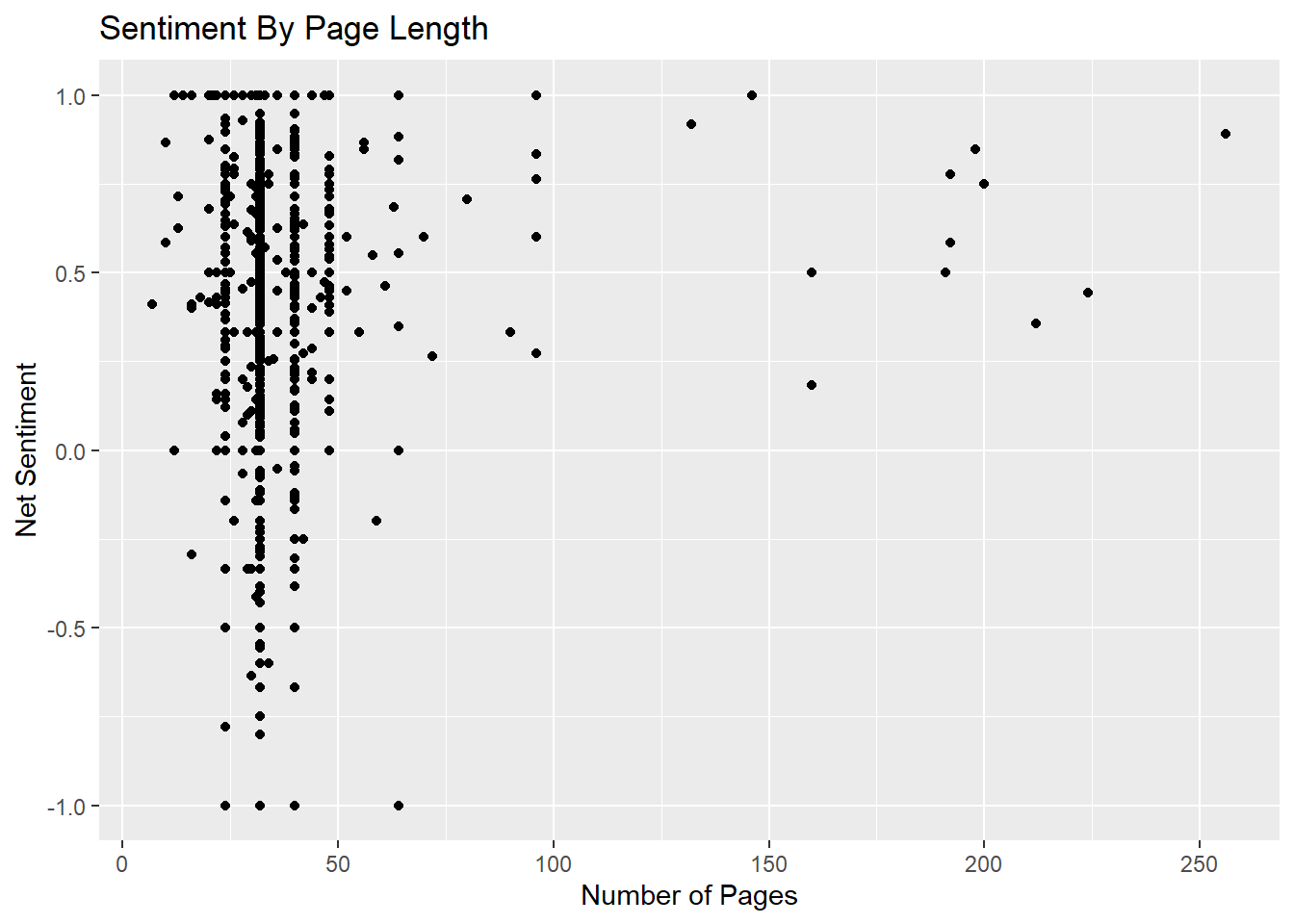
In the chart below, you can see that there appears to be a relationship between longer books and more positive sentiment.
nrcbooks %>%
  mutate(sent = case_when(sent == "Positive Words" ~ 1,
                          sent == "Neutral Words" ~ 0,
                          sent == "Negative Words" ~ -1)) %>%
  group_by(book) %>%
  summarise(NetSentiment = sum(sent)/sum(abs(sent)), TotalSent = n()) %>%
  left_join(booksread, by = c("book"="Title")) %>%
  ggplot(aes(x = NumberOfPages, y = NetSentiment)) +
  geom_point() +
  labs(title = "Sentiment By Page Length", x = "Number of Pages", y = "Net Sentiment")
## Warning: Removed 26 rows containing missing values (geom_point).